Sphere
Object type: Surface
Definition
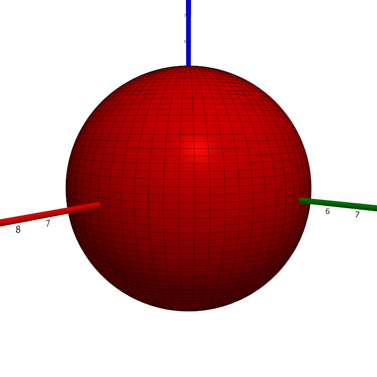
In $\mathbb{R}^3$, a sphere of radius $r > 0$ is the set of points $(x,y,z)$ satisfying $$x^2 + y^2 + z^2 = r^2.$$ If $r = 1$, we have the unit sphere. Below, a sphere of radius 5 is shown.
Parameterisation
The sphere of radius $r$ is obtained as the circle $$C := \left\{(x,y,z)\in\mathbb{R}^3: x^2 + z^2 = r^2 \wedge x \ge 0 \wedge y=0\right\}$$ is rotated about the $z$ axis. This circle may be parameterised in several ways. Indeed, $$C = \mathbf{a}\left(\left[0,\pi\right]\right) = \mathbf{b}\left(\left[-1, 1\right] \right)$$ where $\mathbf{a}: t \mapsto (r\sin t, 0, r\cos t)$ and $\mathbf{b}: t \mapsto \left(r\sqrt{1-u^2}, 0, ru\right)$, as is readily verified. Thus, the sphere of radius $r$ is the image $\mathbf{r}(D)$ where $$\mathbf{r}(\theta, \varphi) = \underline{\mathbf{e}}\begin{pmatrix}r\sin\theta\cos\varphi\\r\sin\theta \sin\varphi\\r\cos\theta\end{pmatrix}$$ and $D := \left[0, \pi\right]\times\left[0, 2\pi\right[$. It is also the image $\mathbf{q}(E)$ where $$\mathbf{q}(u,v) = \underline {\mathbf{e}} \begin{pmatrix}r\sqrt{1-u^2}\cos v\\r\sqrt{1-u^2}\sin v\\ru\end{pmatrix}$$ and $E := \left[-1, 1\right]\times\left[0,2\pi\right[$. The image above shows the parameter curves obtained using $\mathbf{r}$.
Properties (with respect to $\mathbf{r}$)
The properties below are with respect to the parameterisation $\mathbf{r}$ given above.
Parameter-curve tangent vectors
The parameter-curve tangent vectors are $$\mathbf{r}_\theta(\theta,\varphi)=\underline{ \mathbf{e}}\begin{pmatrix}r\cos\theta\cos\varphi\\r\cos\theta\sin\varphi\\-r\sin\theta \end{pmatrix}, \quad\quad \mathbf{r}_\varphi(\theta,\varphi)=\underline{\mathbf{e}} \begin{pmatrix}-r\sin\theta\sin\varphi\\r\sin\theta\cos\varphi\\0\end{pmatrix}.$$
Standard unit normal
The standard unit normal vector field is $$\mathbf{\hat{N}}(\theta,\varphi) = \underline{\mathbf{e}}\begin{pmatrix}\sin\theta\cos\varphi\\\sin\theta\sin\varphi\\\cos \theta\end{pmatrix}.$$
Area element
The area element is $$dA = r^2\sin\theta~d\theta d\varphi.$$
First fundamental form
The first fundamental form of the sphere of radius $r$ is $$\mathcal{F}(\theta, \varphi) = \begin{pmatrix}r^2&&0\\0&&r^2\sin^2\theta\end{pmatrix}.$$
Second fundamental form
The second fundamental form is $$\mathcal{M}(\theta,\varphi) = \begin{pmatrix} -r&&0\\0&&-r\sin^2\theta\end{pmatrix}.$$
Christoffel symbols
The Christoffel symbols are $$\Gamma^1_{\alpha\beta}=\begin{pmatrix}0&&0\\0&&-\frac{1}{2} \sin{2\theta}\end{pmatrix}, \quad\quad \Gamma^2_{\alpha\beta} = \begin{pmatrix}0&&\cot\theta \\\cot\theta&&0\end{pmatrix}.$$
Curvatures
Every point is an umbilic with curvature $$\kappa = -\frac{1}{r}.$$ Therefore, the Gaussian and mean curvatures are $$K = \frac{1}{r^2}, \quad\quad H = -\frac{2}{r},$$ respectively. Notice that the sphere is a surface of constant positive Gaussian curvature.
Properties (with respect to $\mathbf{q}$)
The properties below are with respect to the parameterisation $\mathbf{q}$ given above.
Parameter-curve tangent vectors
The parameter-curve tangent vectors are $$\mathbf{q}_u(u,v) = \underline{\mathbf{e}}\begin {pmatrix}-\frac{ur}{\sqrt{1-u^2}}\cos v\\-\frac{ur}{\sqrt{1-u^2}}\sin v\\r\end{pmatrix},\quad \quad \mathbf{q}_v(u,v) = \underline{\mathbf{e}} \begin{pmatrix}-r\sqrt{1-u^2}\sin v\\r\sqrt {1-u^2}\cos v\\0\end{pmatrix}.$$
Standard unit normal
The standard unit normal vector field is $$\mathbf{\hat{N}}(u,v) = \underline {\mathbf{e}}\begin{pmatrix}-\sqrt{1-u^2}\cos v\\-\sqrt{1-u^2}\sin v\\-u\end{pmatrix}.$$
Area element
The area element is $$dA = r^2 ~dudv.$$ Notice that the area element is constant on the sphere!
First fundamental form
The first fundamental form of the sphere is $$\mathcal{F}(u,v) = \begin{pmatrix}\frac{r^2} {1-u^2}&&0\\0&&r^2 (1-u^2)\end{pmatrix}.$$
Second fundamental form
The second fundamental form is $$\mathcal{M}(u,v) = \begin{pmatrix}\frac{r}{1-u^2}&&0\\0&& r(1-u^2)\end{pmatrix}.$$
Christoffel symbols
The Christoffel symbols are $$\Gamma^1_{\alpha\beta} = u\begin{pmatrix}\frac{1}{1-u^2}&&0\\ 0&&1-u^2\end{pmatrix}, \quad\quad \Gamma^2_{\alpha\beta} = -\frac{u}{1-u^2}\begin{pmatrix}0&&1\\ 1&&0\end{pmatrix}.$$
Curvatures
Every point is an umbilic with curvature $$\kappa = \frac{1}{r}.$$ Therefore, the Gaussian and mean curvatures are $$K = \frac{1}{r^2}, \quad\quad H = \frac{2}{r},$$ respectively. Notice that the sphere is a surface of constant positive Gaussian curvature.
Generalisations
If one applies a linear transformation $\mathbb{R}^3 \rightarrow \mathbb{R}^3$ with matrix $$\begin{pmatrix}a&&0&&0\\0&&b&&0\\0&&0&&c\end{pmatrix}$$ ($a, b, c > 0$) to a sphere centred at the origin, one obtains an ellipsoid that is not a sphere unless $a=b=c$, namely, the ellipsoid $$\left(\frac{x}{a}\right)^2 + \left(\frac{y} {b}\right)^2 + \left(\frac{z}{c}\right)^2 = 1.$$
Trivia
Sphere point-picking
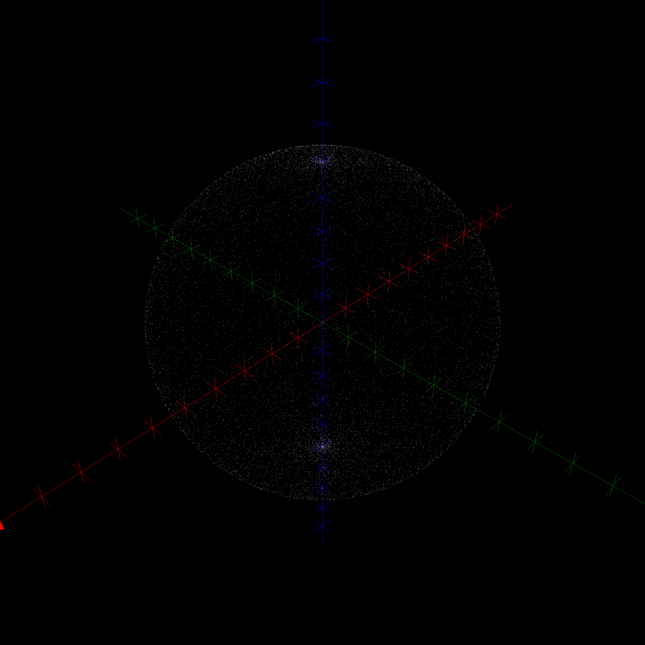
Consider the problem of picking random points on a sphere. By 'random', we mean that for every $\epsilon > 0$ the probability that the point will belong to a geodesic disk of radius $\epsilon$ centered at a given point on the sphere (in $\mathbb{R}^3$) is independent of the centrepoint. It does not do to pick a random point $(\theta,\varphi)\in\left[0,\pi\right]\times\left[0,2\pi\right[$ and take $\mathbf{r}(\theta,\varphi)$, for this will yield too many points near the poles $(0, 0, \pm r)$ of the sphere. This is evident from the area element corresponding to the parameterisation $\mathbf{r}$.
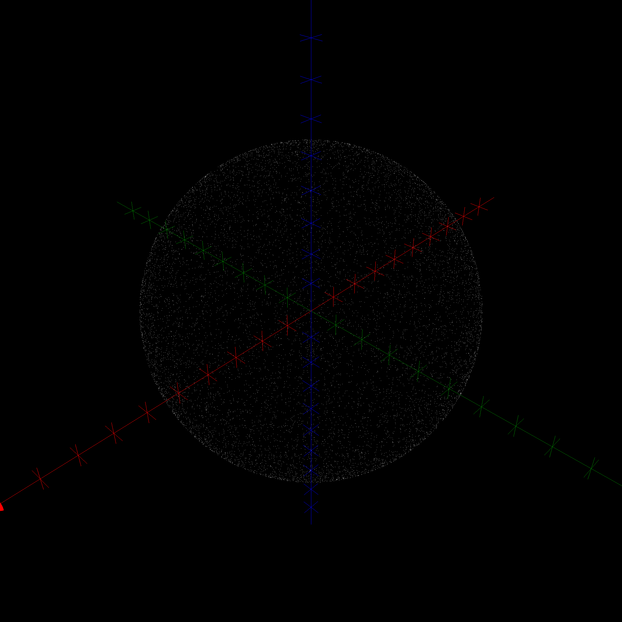
However, it does do to pick a random point $(u,v)\in\left[-1,1\right]\times\left[0,2\pi\right[$ and take $\mathbf{q}(u,v)$, because the area element corresponding to the parameterisation $\mathbf{q}$ is constant. Hence, every parameter-plane region is magnified by the same factor when mapped to the sphere (in terms of surface areas in the parameter plane and the sphere).
Below we show the result of picking 10 000 random points in the respective parameter planes and mapping these to the sphere. Notice the accumulation of points near the poles of the sphere when the map $\mathbf{r}$ is used.