Basic Theory
Curves in the Plane
Perhaps the most used definition of a plane curve is the following: A plane curve $C \subset \R^2$ is the image of some interval $I \subset \R$ under some continuous parameterisation map $\mathbf{r}: I \to \R^2$, that is, $C = \mathbf{r}(I)$. Other (non-equivalent) definitions are based on the fact that every point on a 'curve' has a neighbourhood (on the curve) homeomorphic to some open interval of $\R$. This requires that the curve has no 'endpoints'; in the language of the first definition of a curve, this means that the interval $I$ has to be open. Also, this prohibits self-intersections, which are clearly allowed according to the first definition. In what follows, we will chiefly allow these kinds of behaviour, and use the first definition. However, we will generally demand that parameterisation maps be differentiable and with non-vanishing derivatives.
Describing a Plane Curve
The are several ways of describing a plane curve, one of which consists simply of giving a parameterisation map $\mathbf{r}$. For instance, the unit circle $C = \mathbf{r}(\left[0,2\pi \right[)$ where $$\mathbf{r}(t) = (\cos t, \sin t), \quad\quad \forall t \in \R.$$
Another common way of defining a curve is to give its equation in some coordinate system of the plane. For instance, if $(x,y)$ are the Cartesian coordinates in $\R^2$, then the unit circle $$C = \left\{(x,y)\in\R^2: x^2 + y^2 = 1\right\},$$ and we say that $x^2 + y^2 = 1$ is the equation of the curve. Often, with some abuse of terminology, we even use the word 'curve' for the formal expression $x^2 + y^2 = 1$ itself. Each new coordinate system in the plane brings a new way of describing (and defining) curves. For instance, in polar coordinates $(r, \varphi)$, defined by $$\begin{align}x &= r \cos \varphi\\y &= r \sin \varphi\end{align}$$ with $r \ge 0$ and $\varphi \in \left[0, 2\pi\right[$, the unit circle has the particularly simple equation $r = 1$.
A (continuous) function $f : D_f \to \R$ with domain $D_f$ a real interval induces a plane curve, namely, its graph $$C = \left\{(x,y) \in \R: x \in D_f \wedge y=f(x) \right\}.$$ This curve can clearly also be stated in terms of its equation $y = f(x)$ and in terms of the parameterisation map $\mathbf{r}: D_f \to \R^2 : t \mapsto (t, f(t)).$ Notice that this is a very restricted way of describing curves; for instance, the unit circle is not the graph of any function.
Finally, any (continuous) scalar field $F : D_F \to \R$ defined in some (nice) region $D_F \subset \R^2$ gives rise to a family of curves, namely, the level curves $$C_\ell = \left\{(x,y) \in D_F: F(x,y) = \ell \right\}, \quad\quad \forall \ell \in R_F$$ where $R_F = F(D_F)$ is the range of $F$. For instance, the unit circle is the level curve $C_1$ of the scalar field $F: \R^2 \to \R: (x,y) \mapsto x^2 + y^2$.
Curvature
By definition, the curvature of a plane curve is the norm of the second derivative (the acceleration) of a 'unit-speed' parameterisation map of the curve; hence, the curvature is a local property, defined pointwise along the curve. A 'unit-speed' parameterisation map is simply a map the derivative of which (the velocity) is of unit norm. Given a curve $C = \mathbf{r}(I)$ with any parameterisation map $\mathbf{r}$ (unit-speed or not), it is straightforward to show that the curvature at parameter value $t$ is $$\kappa(t) = \frac{|\mathbf{ \dot r}(t)\times\mathbf{\ddot r}(t)|}{|\mathbf{\dot r}(t)|^3}, \quad\quad \forall t\in I.$$ It can also be shown that the curvature is the absolute value of the rate-of-change of the angle between the curve's tangent vector and the positive $x$ axis with respect to arc length. This rate of change, with its sign, is called the signed curvature of the curve.
Curves in Space
Similarly, a curve in space can either be defined as the image of a (continuous) parameterisation map $\mathbf{r}: I \to \R^3$, or by demanding that every point on it should have a neighbourhood homeomorphic to some open subset of $\R$.
Describing a Space Curve
Of course, one can describe a space curve by giving a parameterisation map. One can also give a pair of equations (in the spatial coordinates) that are to hold simultaneously; in this case, the curve is the intersection of two surfaces. For example, the unit circle in the $xy$ plane is the image $C = \mathbf{r}(\left[0,2\pi\right[)$ where $$\mathbf{r}(t) = (\cos t, \sin t, 0), \quad\quad\forall t\in\R,$$ but it is also the set $$C = \left\{(x,y,z)\in\R^3: x^2 + y^2 = 1, z = 0 \right\},$$ that is, it is the intersection between the cylinder $x^2 + y^2 = 1$ and the plane $z = 0$. Again, every spatial coordinate system yields a new way of describing space curves. For instance, in cylindrical coordinates $(r,\varphi,z)$, defined by $$\begin{align}x &= r \cos \varphi\\y &= r \sin \varphi\\z &= z\end{align}$$ and $r \ge 0, \varphi \in \left[0,2\pi\right[$, the same curve has equations $r = 1, z = 0$ (where each individual equation retains its previous interpretation, i.e., as a cylinder and a plane, respectively).
Curvature
By definition, the curvature of a space curve is the norm of the second derivative (the acceleration) of a unit-speed parameterisation map of the curve; hence, the curvature is a local property, defined pointwise along the curve. Given a curve $C = \mathbf{r}(I)$ with any parameterisation map $\mathbf{r}$ (unit-speed or not), it is straightforward to show that the curvature at parameter value $t$ is $$\kappa(t) = \frac{|\mathbf{ \dot r}(t)\times\mathbf{\ddot r}(t)|}{|\mathbf{\dot r}(t)|^3}, \quad\quad \forall t\in I.$$
Tangent, Normal, and Binormal
Given a curve $C = \mathbf{r}(I)$ with $\mathbf{r}$ unit-speed, the unit tangent vector at $t \in I$ is $$\mathbf{\hat t}(t) = \mathbf{\dot r}(t).$$ Although $\mathbf{\hat t}(t)$ depends upon the actual parameterisation map $\mathbf{r}$ (namely, upon the orientation of the curve), the set $\left\{\mathbf{\hat t}(t), -\mathbf{\hat t}(t)\right\}$ is independent of parameterisation function at corresponding points on the curve. The standard unit normal vector is $$\mathbf{\hat n}(t) = \frac{1}{|\mathbf{\ddot r}(t)|}\mathbf{\ddot r}(t) = \frac{1}{\kappa(t)}\mathbf{\ddot r}(t).$$ This vector is independent of parameterisation, and it is obviously only well-defined at points of non-vanishing curvature. Since $\mathbf{r}$ is unit-speed, $\mathbf{\hat t}(t) \perp \mathbf{\hat n}(t)$ for every $t\in I$, and so by adding a third vector $$\mathbf{\hat b}(t) =\mathbf{\hat t}(t)\times\mathbf{\hat n}(t),$$ the so-called binormal vector (which is also clearly seen to be unit), we have in fact a natural basis $\mathbf{\hat t}(t), \mathbf{\hat n}(t), \mathbf{\hat b}(t)$ of $\R^3$ at each $t \in I$ for which $\kappa(t) \ne 0$.
Torsion
Intuitively, the torsion of a space curve is a measure of the amount by which the curve 'fails' to lie within a single plane, locally. Specifically, the torsion $\tau$ is defined by $\mathbf{\hat b}\prime = −\tau \mathbf{\hat n}$ where $\mathbf{\hat n}$ and $\mathbf{\hat b}$ are the standard unit normal and standard unit binormal of some unit-speed parameterisation of the curve. It can be shown that, given any curve $C = \mathbf{r}(I)$, with $\mathbf{r}$ not necessarily unit-speed, the torsion is $$\tau(t) = \frac {(\mathbf{\dot r}(t)\times\mathbf{\ddot r}(t))\cdot \mathbf{\dddot r}(t)}{|\mathbf{\dot r}(t)\times\mathbf{\ddot r}(t)|^2}, \quad\quad \forall t\in I: \kappa(t) \ne 0.$$
Surfaces
Not surprisingly, there are pricipally two common ways of defining the concept of a (two-dimensional) surface (in $\R^3$). Either, one may define a surface as the image of some (nice) parameter-plane region $U \subset \R^2$ under a (continuous) parameterisation function $\mathbf{r}: U \to \R^3$, or one may define a surface as a subset $S \subset \R^3$ such that every point on the 'surface' has a neighbourhood (on the surface) homeomorphic to some open disk in $\R^2$. Essentially the same remarks can be made here as we did in the case of curves, namely, the latter approach cannot allow surfaces with 'edges' (so $U$ has to be open) and nor can it allow self-intersections. We will mainly use the first approach. We will, however, make the standard requirements that the parameterisation maps $\mathbf{r}$ be continuously differentiable, and that the derivatives $\mathbf{r}_u(u,v)$ and $\mathbf{r}_v(u,v)$ be linearly independent at every point $(u,v)\in U$.
Describing a Surface
Of course, a particular surface can be defined by a suitable parameterisation map $\mathbf{r}: U \to \R^3$. For instance, the unit sphere is the image $\mathbf{r}(U)$ where $$\mathbf{r}(\theta,\varphi) = \basis\begin{pmatrix} \sin\theta\cos\varphi\\\sin\theta\sin\varphi\\\cos\theta\end{pmatrix}, \quad\quad\forall (\theta, \varphi)\in U$$ and $U := \left[0, \pi\right]\times \left[0,2\pi\right[$. Since a surface in $\R^3$, like a curve in $\R^2$, is an object of codimension $1$, it can also be specified by an equation. For instance, the unit sphere is $$S = \left\{(x,y,z)\in\R^3: x^2 + y^2 + z^2 = 1\right\},$$ and we say that $x^2 + y^2 +z^2 = 1$ is the equation of the surface. Often, with some abuse of terminology, we even use the word 'surface' for the formal expression $x^2 + y^2 + z^2 = 1$ itself. Each new coordinate system in space brings a new way of describing (and defining) surfaces. For instance, in spherical coordinates $(r, \theta, \varphi)$, defined by $$\begin{align}x &= r \sin \theta \cos \varphi\\y &= r \sin \theta \sin \varphi\\z &= r \cos \theta\end{align}$$ with $r \ge 0$, $\theta \in \left[0,2\pi\right]$, and $\varphi \in \left[0,2\pi\right[$, the unit sphere has the particularly simple equation $r = 1$.
Given a (continuous) function $f : D_f \to \R$ with (nice) domain $D_f \subset \R^2$, its graph is the surface $$S = \left\{(x,y,z) \in \R^3: (x,y) \in D_f \wedge z=f(x,y)\right\}.$$ Clearly, this surface can also be given by its eqation $z = f(x,y)$ and by the parameterisation map $\mathbf{r}: D_f \to \R^3: (x,y) \mapsto (x, y, f(z))$. Analogous to the case of curves in the plane, this is a very restricted way of describing a surface; for example, the unit sphere is not the graph of any function.
Finally, given any (continous) scalar field $F: D_F \to \R$ defined in some (nice) domain $D_F \subset \R^3$, the level surfaces belong to the family of surfaces $$S_\ell = \left\{(x,y,z)\in D_F: F(x,y,z) = \ell\right\}, \quad\quad\forall \ell\in R_F$$ where $R_F=F(D_F)$ is the range of $F$. For example, the unit sphere is the level surface $S_1$ of the scalar field $\mathbf{r}: \R^3 \to \R: (x,y,z) \mapsto x^2+y^2+z^2$.
Properties of Surfaces
Let $S = \mathbf{r}(U)$ be a surface. At every coordinate $(u,v)\in U$, $\mathbf{r}_u(u,v)$ and $\mathbf{r}_v(u,v)$ forms a basis of the tangent space of $S$ at $\mathbf{r}(u,v)$. The plane $$\Pi_{(u,v)} = \left\{(x,y,z)\in\R^3: (x,y,z) = \mathbf{r}(u,v) + s\mathbf{r}_u(u,v) +t\mathbf{r}_v(u,v)\right\}$$ is called the tangent plane of $S$ at $\mathbf{r}(u,v)$, and is independent of the choice of parameterisation function $\mathbf{r}$. Below, a tangent plane on the unit sphere is shown.
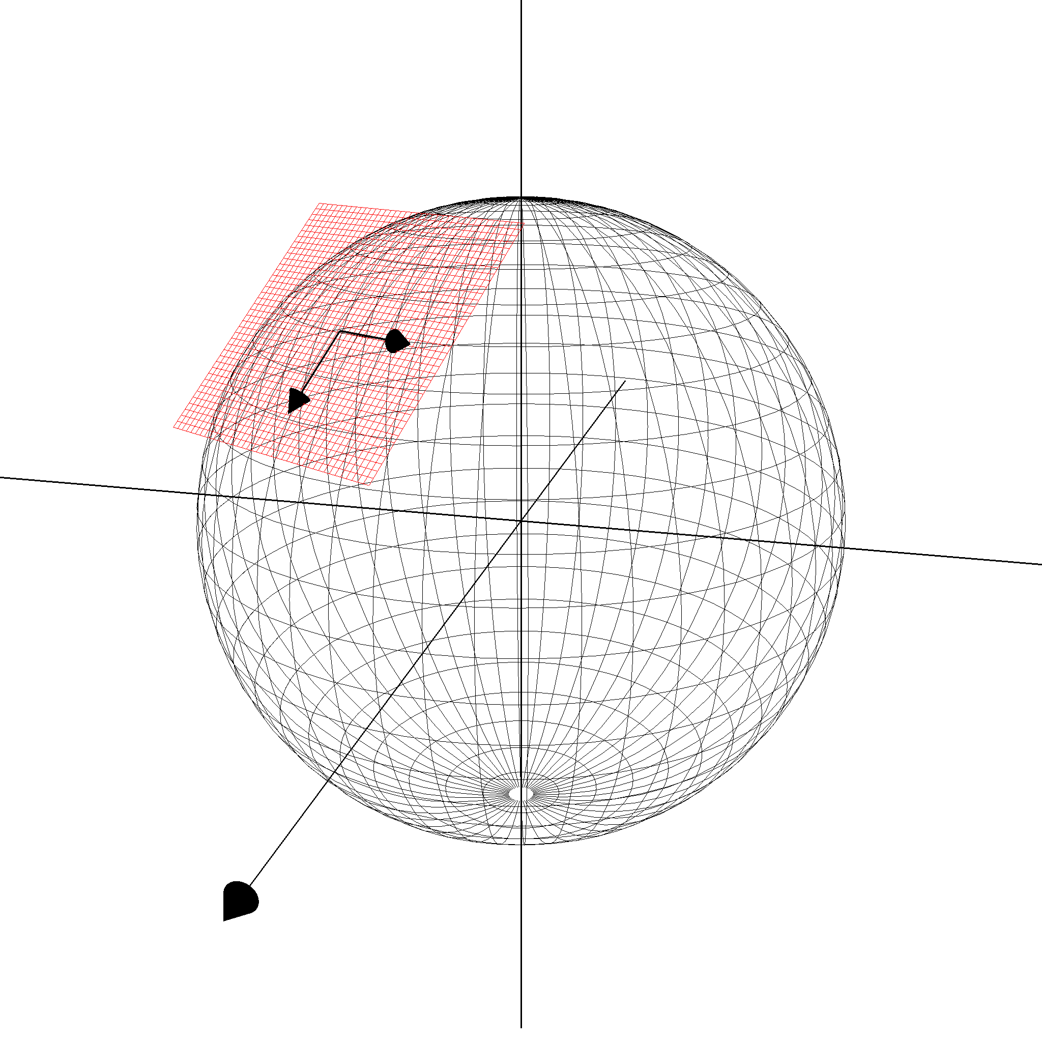
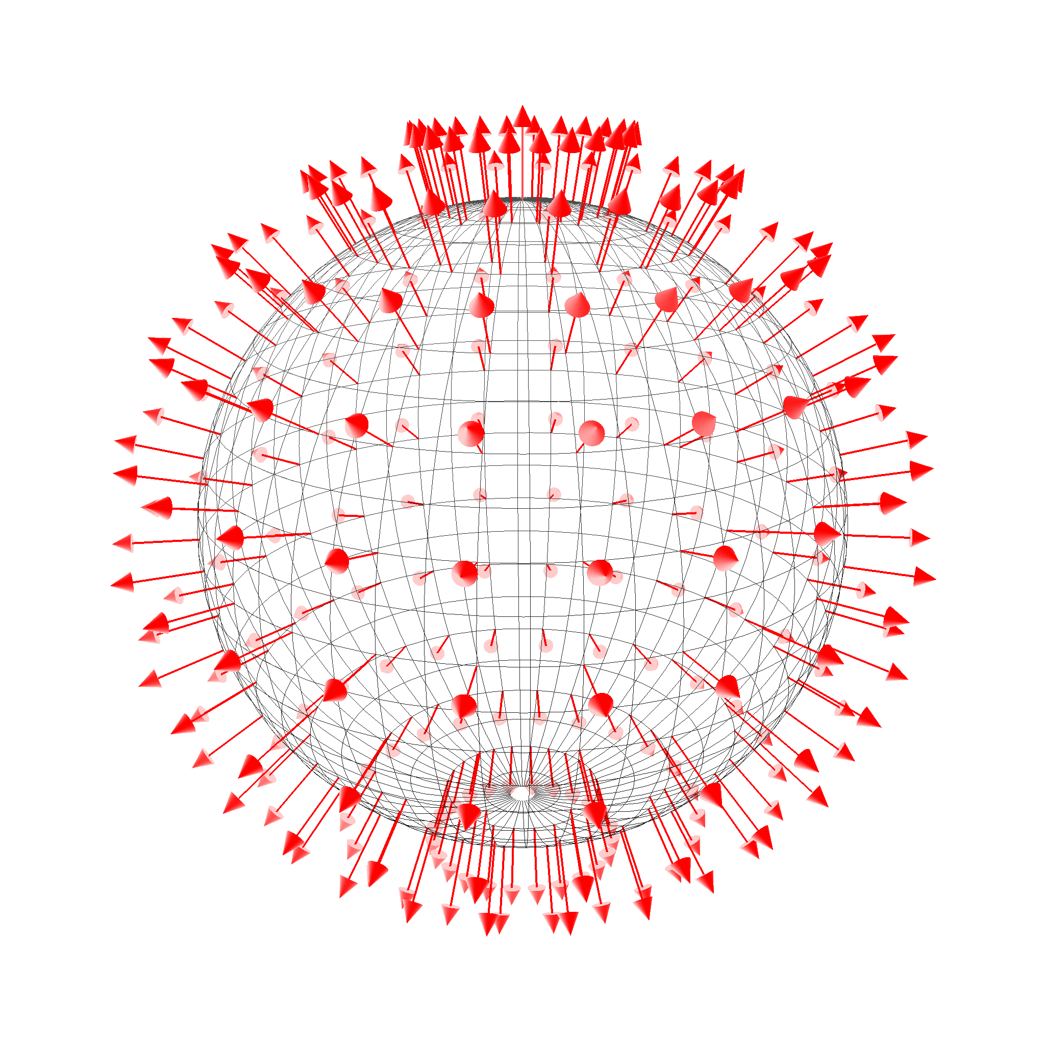
The vector field $$\mathbf{\hat N}(u,v) = \frac{1}{|\mathbf{r}_u(u,v) \times \mathbf{r}_v(u,v)|} \mathbf{r}_u(u,v) \times \mathbf{r}_v(u,v), \quad\quad\forall(u,v)\in U$$ is called the standard unit normal vector field of the surface, and, up to the sign of the vectors, it is independent of the particular choice of parameterisation map as long as the surface is orientable. Below, the normal vector field on the unit sphere is shown.
Curves on Surfaces. Parameter Curves
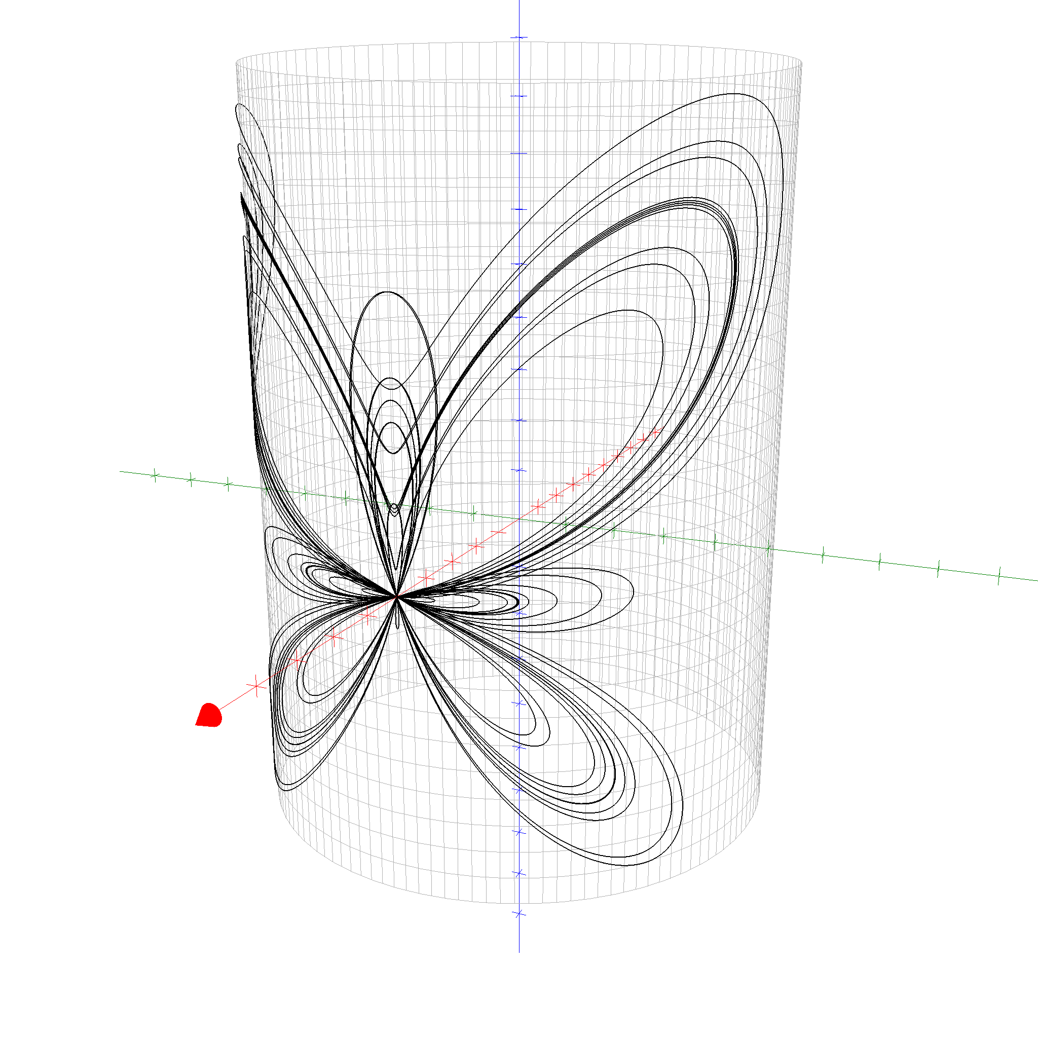
Consider a surface $S = \mathbf{r}(U)$, and a curve $\gamma = \mathbf{p}(I) \subset U$ in the parameter-plane region $U$ of $S$. Then the image $C = \mathbf{r}(\gamma) = (\mathbf{r}\circ\mathbf{p})(I) \subset S$ is a space curve on the surface $S$. For example, one can draw the butterfly curve on a cylinder:

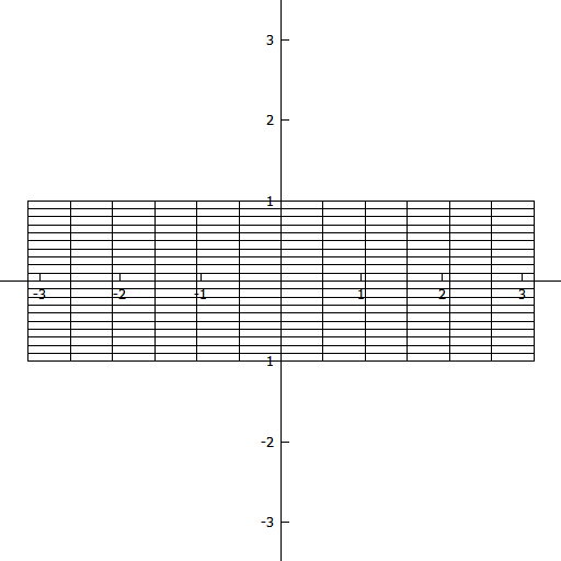
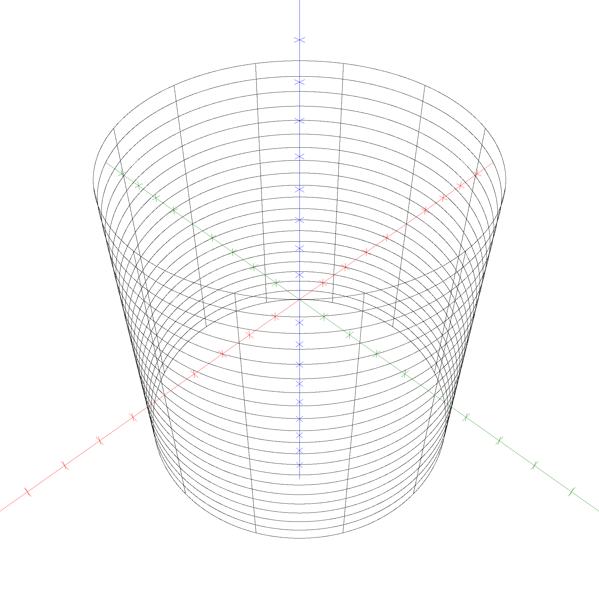
In fact, in all the pictures of surfaces given above, we have not plotted the surfaces themselves, but rather the so-called parameter curves of the surfaces, that is, the images of rectangular grids in the parameter planes. Below a rectangular grid $G \subset U = \left[-\pi,\pi\right[\times\left[-1,1\right]$ is shown, together with its image $\mathbf{r}(G)$ where $\mathbf{r}(u,v) = 5(\cos u,\sin u,v)$ parameterizes a cylinder.